Modern Portfolio Theory

Introduction

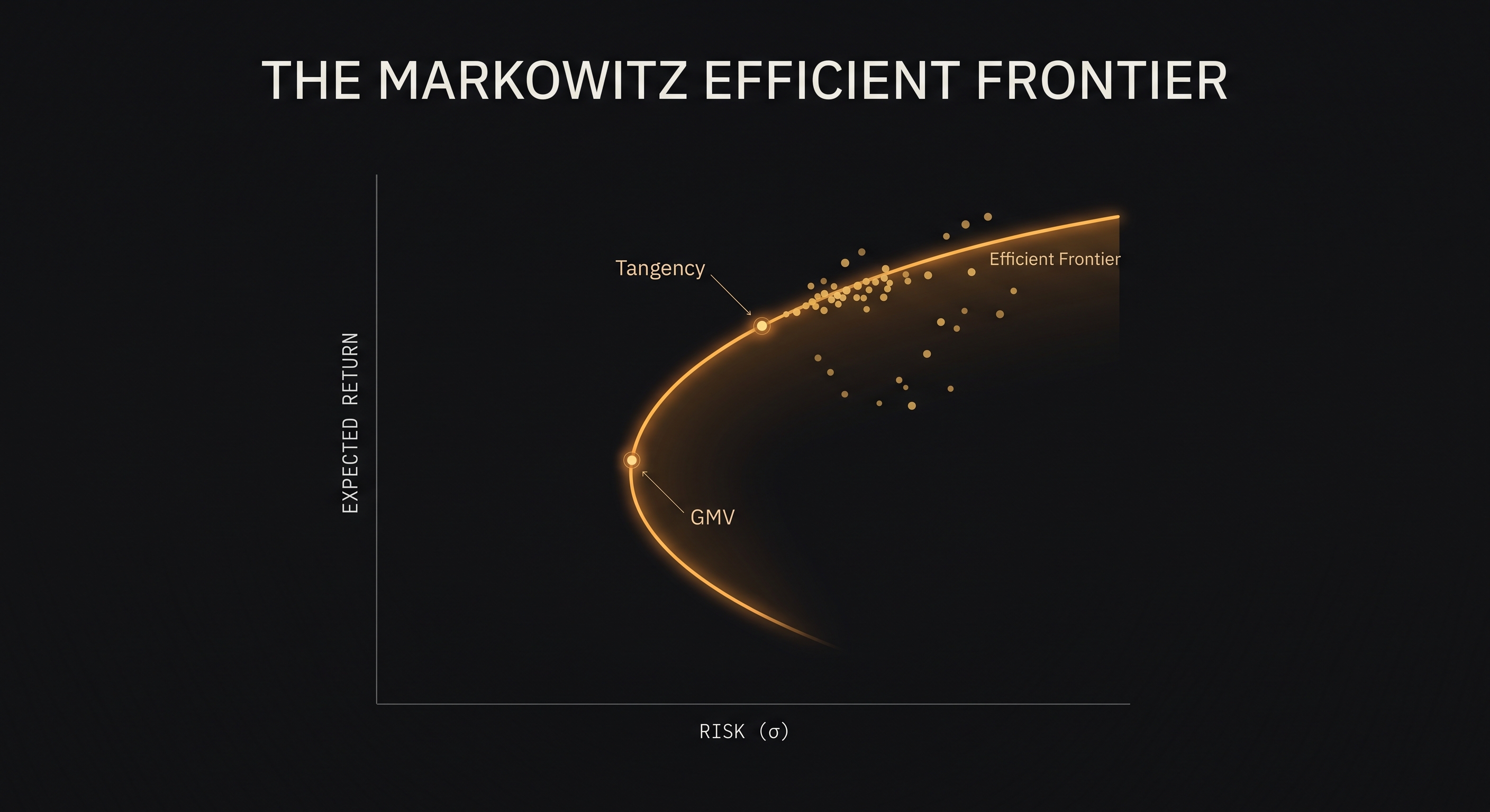
Markowitz Portfolio Selection is a part of the Modern Portfolio Theory, formulated in 1952 by Harry Markowitz, published in The Journal of Finance. It states that it is possible to find the most optimal combination, for a specific set of stocks, to compose a portfolio. The proportions can be found by modeling the stocks' risk/return relation. Markowitz's work is the exact method that allows one to effectively compute how risk/return interact to find the best composition — maximizing return for a specific risk.

The main pillars, explained in details later, that — together — obtain the optimal portfolio are:

• Expected Return ($E \lbrack R_p \rbrack$)
• Standard Deviation / Risk / Volatility ($\sigma_p$)
• Beta ($\beta$)
• The Sharpe Ratio ($\text{SR}(w)$)

The requirements to understand this theory properly are basic knowledge on probability and linear algebra, anything else can be built on this foundation.

Expected Return ($E\lbrack R_p \rbrack$)

Just like as the naming already suggests, it's the anticipated average profit (either positive — effectively a profit —, or negative — effectively a loss).

For a single asset, this metric is commonly estimated using the historical average returns or forward-looking financial models.

For an entire portfolio, it is the weighted average of the expected return of all individuals assets inside of it:

$$E \lbrack R_p \rbrack = \sum_{i=1}^n w_i E \lbrack R_i \rbrack$$

Standard Deviation / Risk / Volatility ($\sigma_p$)

As the name suggests, standard deviation quantifies how far a portfolio's returns typically stray from their expected value — it is Markowitz's chosen proxy for risk. It is not computed as a simple weighted average of each asset's own volatility, but through the full covariance structure between every pair of assets in the portfolio:

$$\sigma_p^2 = \sum_{i=1}^n \sum_{j=1}^n w_i w_j \sigma_{ij}, \qquad \sigma_p = \sqrt{\sigma_p^2}$$

where $\sigma_{ij}$ is the covariance between the returns of assets $i$ and $j$ ($\sigma_{ii} = \sigma_i^2$, the variance of asset $i$ on its own). It is, for exactly this reason, the equation where diversification actually earns its keep: portfolio standard deviation is bounded above by the weighted average of the individual assets' standard deviations,

$$\sigma_p \le \sum_{i=1}^n w_i \sigma_i,$$

with equality only when every pair of assets is perfectly correlated ($\rho_{ij} = 1$ for all $i,j$). Away from that boundary case, the inequality is strict — risk reduced below what a naive weighted average would suggest, without giving up any expected return.

Beta ($\beta$)

Beta doesn't come from Markowitz's original 1952 paper — it was formalized twelve years later, in 1964, within the Capital Asset Pricing Model developed independently by Sharpe, Lintner, and Mossin, building directly on Markowitz's mean-variance framework. It answers a question that framework leaves open on its own: how much of an asset's risk is unique to it, and how much is simply the price of being in the market at all.

Beta measures how sensitive an asset's — or a portfolio's — returns are to movements in the broader market. That sensitivity is formalized as a ratio: the covariance between the asset's returns and the market's returns, divided by the market's own variance.

$$\beta_i = \frac{\text{Cov}(R_i, R_m)}{\text{Var}(R_m)} = \frac{\sigma_{im}}{\sigma_m^2}$$

This ratio is what the single-index model uses to split an asset's total variance into two very different components:

$$\sigma_i^2 = \underbrace{\beta_i^2 \sigma_m^2}_{\text{systematic}} + \underbrace{\sigma_{\epsilon_i}^2}_{\text{idiosyncratic}}$$

the diversifiable, asset-specific noise ($\sigma_{\epsilon_i}^2$) that a well-built portfolio washes out, and the market-wide risk ($\beta_i^2 \sigma_m^2$) that no amount of diversification can touch. That undiversifiable remainder is precisely what beta is built to price — a single number for the risk an investor cannot escape simply by holding more stocks. A portfolio's beta, in turn, is just the weighted average of its constituents' betas: $\beta_p = \sum_{i=1}^n w_i \beta_i$.

The Sharpe Ratio ($\text{SR}(w)$)

$$\text{SR}(w) = \frac{E \lbrack R_p \rbrack - R_f}{\sigma_p}$$

Introduced by William Sharpe in 1966 — originally under the far clunkier name reward-to-variability ratio — the Sharpe Ratio is the natural synthesis of the first three pillars: a single number for risk-adjusted performance. Sharpe revisited the measure himself in a 1994 paper titled, fittingly, The Sharpe Ratio, which is where the name actually stuck. It measures how much return a portfolio earns above the risk-free rate, $R_f$, for every unit of volatility, $\sigma_p$, an investor has to tolerate to earn it. It rewards efficiency rather than raw magnitude: two portfolios with identical expected return are not equally desirable if one gets there with far less risk. It also becomes the natural objective function once a risk-free asset is introduced alongside Markowitz's frontier — the extension known as the Capital Market Line: sweeping across every feasible set of weights $w$ on the risky assets and keeping the one that maximizes $\text{SR}(w)$ identifies the tangency portfolio, the point on the efficient frontier every rational investor combines with the risk-free asset (Tobin's separation theorem).

Conclusion

That tangency portfolio builds directly on the frontier Markowitz described in 1952 — it is the concrete answer to a question his framework leaves open until a risk-free asset enters the picture: for a given universe of risky assets, which single combination maximizes return for the risk one is willing to bear? That answer only exists because expected return, standard deviation, and beta are computed jointly rather than independently — each pillar constraining, and constrained by, the other two. That interdependence is, in the end, exactly what Markowitz Portfolio Selection formalizes: not a checklist of four numbers, but one mutually consistent optimization problem.